Getting Started

In this section, we will explaine some of the basics of the CameraTransform package.

Using Cameras

The most important object is the Camera.

It can be created with different projections (for normal cameras: RectilinearProjection or pamoranic cameras: CylindricalProjection, EquirectangularProjection).

We define the camera parameters and create a camera with the rectinilar projection (default pin-hole camera) and the spatial orientation, 10m above ground and looking down 45°. Keep in mind the orientation of the tilt angle, where a 0° tilt angle corresponds to a view perpedicular on the ground plane

import cameratransform as ct

# intrinsic camera parameters
f = 6.2    # in mm
sensor_size = (6.17, 4.55)    # in mm
image_size = (3264, 2448)    # in px

# initialize the camera
cam = ct.Camera(ct.RectilinearProjection(focallength_mm=f,
                                         sensor=sensor_size,
                                         image=image_size),
               ct.SpatialOrientation(elevation_m=10,
                                     tilt_deg=45))

Tip

For a more detailed explanation of how the camera orientation parameters (elevation, tilt, roll, heading, x, y) are defined, see Camera Orientation.

Tip

For a more detailed explanation of how the camera projection parameters (sensor, image, focallength_mm) are defined, see Projections.

We can also omit the SpatialOrientation and later change the parameters:

cam.elevation_m = 34.027
cam.tilt_deg = 83.307926
cam.roll_deg = -1.916219

With the camera object we can project 3D world points (space coordinate system, in meters) to the 2D image pixels (image coordinate system, in pixels).

cam.imageFromSpace([3.17, 8, 0])

array([ 2807.03150016, 10239.20837453])

The routines take lists and 1D numpy arrays or, to transform multiple points at once, stacked lists or 2D numpy arrays. As the calculations are internally handled as vectorized numpy calculations, transforming multiple points in one go is advantagous.

cam.imageFromSpace([[3.17, 8, 0],
                    [3.17, 8, 10],
                    [4.12, 10, 0],
                    [4.12, 10, 10]])

array([[ 2807.03150016, 10239.20837453],
       [ 2833.09367445,  8187.05449921],
       [ 2861.32478822,  8888.15694679],
       [ 2888.29025648,  7032.51227791]])

Or the other way around, from image to space. This transformation is not unique, as the information on how far the object was away from the camera is lost when transforming from space to the image. Therefore, an additional constraint has to be supplied when performing this back-transformation. The default is to require \(Z=0\).

cam.spaceFromImage([2445, 1569])

array([ 36.26041556, 145.50056995,   0.        ])

cam.spaceFromImage([2445, 1569], X=10)

array([10.        , 40.12655887, 24.64293766])

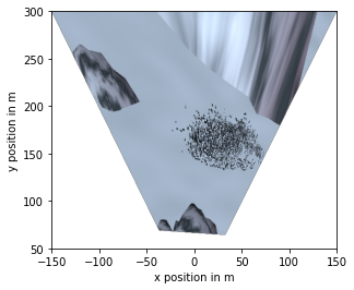
Often it is also advantagouse to have a top vie projection of the camera image. This can be done using the Camera.getTopViewOfImage() method. The extend of the top view in meters can be specified and the resolution (how many pixels per meter). As a convienience, the image can be plotted directly.

%matplotlib inline
import matplotlib.pyplot as plt
# display a top view of the image
im = plt.imread("CameraImage.jpg")
top_im = cam.getTopViewOfImage(im, [-150, 150, 50, 300], scaling=0.5, do_plot=True)
plt.xlabel("x position in m")
plt.ylabel("y position in m");

Tip

As CameraTransform cannot detect the occlusions, the top view projection is not a real top view, any extended object will cast a "projection shadow" on everything behind it.

Fitting

This section will cover the basics for estimating the camera parameters from information in the image.

First we define the camera with a focal length and the image size obtained from a loaded image.

import cameratransform as ct
import numpy as np
import matplotlib.pyplot as plt

im = plt.imread("CameraImage2.jpg")
camera = ct.Camera(ct.RectilinearProjection(focallength_px=3863.64, image=im))

CameraTransform provides different methods to provide the fitting routine with information.

The camera elevation, tilt (and roll) can be fitted using objects of known height in the image that stand on the Z=0 plane. We call the Camera.addObjectHeightInformation() method with the pixel positions of the feed points, head points, the height of the objects, and the standard deviation of the height distribution.

feet = np.array([[1968.73191418, 2291.89125757], [1650.27266115, 2189.75370951], [1234.42623164, 2300.56639535], [ 927.4853119 , 2098.87724083], [3200.40162013, 1846.79042709], [3385.32781138, 1690.86859965], [2366.55011031, 1446.05084045], [1785.68269333, 1399.83787022], [ 889.30386193, 1508.92532749], [4107.26569943, 2268.17045783], [4271.86353701, 1889.93651518], [4007.93773879, 1615.08452509], [2755.63028039, 1976.00345458], [3356.54352228, 2220.47263494], [ 407.60113016, 1933.74694958], [1192.78987735, 1811.07247163], [1622.31086201, 1707.77946355], [2416.53943619, 1775.68148688], [2056.81514201, 1946.4146027 ], [2945.35225814, 1617.28314118], [1018.41322935, 1499.63957113], [1224.2470045 , 1509.87120351], [1591.81599888, 1532.33339856], [1701.6226147 , 1481.58276189], [1954.61833888, 1405.49985098], [2112.99329583, 1485.54970652], [2523.54106057, 1534.87590467], [2911.95610793, 1448.87104305], [3330.54617013, 1551.64321531], [2418.21276457, 1541.28499777], [1771.1651859 , 1792.70568482], [1859.30409241, 1904.01744759], [2805.02878512, 1881.00463747], [3138.67003071, 1821.05082989], [3355.45215983, 1910.47345815], [ 734.28038607, 1815.69614796], [ 978.36733356, 1896.36507827], [1350.63202232, 1979.38798787], [3650.89052382, 1901.06620751], [3555.47087822, 2332.50027861], [ 865.71688784, 1662.27834394], [1115.89438493, 1664.09341647], [1558.93825646, 1671.02167477], [1783.86089289, 1679.33599881], [2491.01579305, 1707.84219953], [3531.26955813, 1729.08486338], [3539.6318973 , 1776.5766387 ], [4150.36451427, 1840.90968707], [2112.48684812, 1714.78834459], [2234.65444134, 1756.17059266]])
heads = np.array([[1968.45971142, 2238.81171866], [1650.27266115, 2142.33767714], [1233.79698528, 2244.77321846], [ 927.4853119 , 2052.2539967 ], [3199.94718145, 1803.46727222], [3385.32781138, 1662.23146061], [2366.63609066, 1423.52398752], [1785.68269333, 1380.17615549], [ 889.30386193, 1484.13026407], [4107.73533808, 2212.98791584], [4271.86353701, 1852.85753597], [4007.93773879, 1586.36656606], [2755.89171994, 1938.22544024], [3355.91105749, 2162.91833832], [ 407.60113016, 1893.63300333], [1191.97371829, 1777.60995028], [1622.11915337, 1678.63975025], [2416.31761434, 1743.29549618], [2056.67597009, 1910.09072955], [2945.35225814, 1587.22557592], [1018.69818061, 1476.70099517], [1224.55272475, 1490.30510731], [1591.81599888, 1510.72308329], [1701.45016126, 1460.88834824], [1954.734384  , 1385.54008964], [2113.14023137, 1465.41953732], [2523.54106057, 1512.33125811], [2912.08384338, 1428.56110628], [3330.40769371, 1527.40984208], [2418.21276457, 1517.88006678], [1770.94524662, 1761.25436746], [1859.30409241, 1867.88794433], [2804.69006305, 1845.10009734], [3138.33130864, 1788.53351052], [3355.45215983, 1873.21402971], [ 734.49504829, 1780.27688131], [ 978.1022294 , 1853.9484135 ], [1350.32991656, 1938.60371039], [3650.89052382, 1863.97713098], [3556.44897343, 2278.37901052], [ 865.41437575, 1633.53969555], [1115.59187284, 1640.49747358], [1558.06918395, 1647.12218082], [1783.86089289, 1652.74740383], [2491.20950909, 1677.42878081], [3531.11177814, 1696.89774656], [3539.47411732, 1745.49398176], [4150.01023142, 1803.35570469], [2112.84669376, 1684.92115685], [2234.65444134, 1724.86402238]])

camera.addObjectHeightInformation(feet, heads, 0.75, 0.03)

If a horizon is visible in the image, it can also be used to fit elevation, tilt (and roll) of the camera. Therefore, we call the Camera.addHorizonInformation() method with the pixel positions of points on the horizon and an uncertaintiy value how many pixels we expect horizon to deviate from the position we provided.

horizon = np.array([[418.2195998, 880.253216], [3062.54424509, 820.94125636]])
camera.addHorizonInformation(horizon, uncertainty=10)

If we know the gps positions of landmarks in the image we can also use them to obtain camera parameters. These also allow to fit the heading angle of the camera. But for gps positions to be meaningful, we have to set the gps position of the camera first (they could also be fitted, if they are unknown).

We call the method Camera.addLandmarkInformation() and provide the pixel coordinates of the landmarks in the image, the positions of these landmarks in the space coordinate system, and an uncertainity value, here we use ±3m for latitude and longitude and ±5m for the height information of the landmarks.

camera.setGPSpos("66°39'53.4\"S  140°00'34.8\"")

lm_points_px = np.array([[2091.300935, 892.072126], [2935.904577, 824.364956]])
lm_points_gps = ct.gpsFromString([("66°39'56.12862''S  140°01'20.39562''", 13.769),
                                  ("66°39'58.73922''S  140°01'09.55709''", 21.143)])
lm_points_space = camera.spaceFromGPS(lm_points_gps)

camera.addLandmarkInformation(lm_points_px, lm_points_space, [3, 3, 5])

CameraTransform stores all these information and creates a log probability value from all information. This log probability can now be used to estimate the camera parameters using metropolis sampling (Camera.metropolis()).

The sampling uses pymc2 statistical objects for the parameters. The parameters need to have the names that the different parts of the camera use. For reference see the chapters on Lens Distortion, Projections, Spacial Orientation, and GPS position.

trace = camera.metropolis([
        ct.FitParameter("elevation_m", lower=0, upper=100, value=20),
        ct.FitParameter("tilt_deg", lower=0, upper=180, value=80),
        ct.FitParameter("heading_deg", lower=-180, upper=180, value=90),
        ct.FitParameter("roll_deg", lower=-180, upper=180, value=0)
        ], iterations=1e4)

100%|██████████| 10000/10000 [00:39<00:00, 255.79it/s, acc_rate=0.128, factor=0.0266]

      elevation_m   tilt_deg  heading_deg  roll_deg   probability
0       21.665337  81.346279   101.617372 -2.281913 -18238.261616
1       21.651165  81.354980   101.634098 -2.254086 -18233.284405
2       21.651165  81.354980   101.634098 -2.254086 -18233.284405
3       21.651165  81.354980   101.634098 -2.254086 -18233.284405
4       21.651165  81.354980   101.634098 -2.254086 -18233.284405
...           ...        ...          ...       ...           ...
8994    20.693984  81.475563   101.621223 -2.330351 -18213.063424
8995    20.693984  81.475563   101.621223 -2.330351 -18213.063424
8996    20.693984  81.475563   101.621223 -2.330351 -18213.063424
8997    20.693984  81.475563   101.621223 -2.330351 -18213.063424
8998    20.693984  81.475563   101.621223 -2.330351 -18213.063424

[8999 rows x 5 columns]

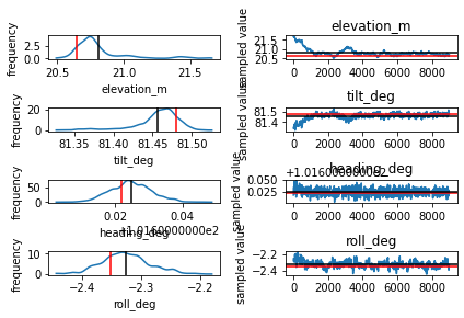
The camera internally stores the trace object and can plot it (Camera.plotTrace()). The trace plot show on the left side the estimated probability distribution for every parameter and on the right side the trace through the sampling space. The sampler provided a good result if the traces fluctuate uncorrelatedly around their central value.

camera.plotTrace()
plt.tight_layout()

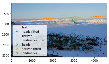
For a visial estimate how correct the most probable value destribes the provided information, the method Camera.plotFitInformation() can be used. It takes the source image as an argument and uses the stored fit information plot plot all data.

camera.plotFitInformation(im)
plt.legend();